Algebraic Programming (ALP) Tutorial
December 2, 2025
Contents
1 Introduction
ALgebraic Programming, or ALP for short, encompasses software technologies that allow programming with explicit
algebraic structures combined with their automated parallelisation and optimisation. This document is a tutorial to the
C++ interface to ALP distributed at https://github.com/Algebraic-Programming/ALP. This framework
supports various interfaces, including ALP/GraphBLAS, ALP/Dense, ALP/Pregel, and a so-called transition path for
sparse linear solvers. ALP provides mechanisms by which auto-parallelisation of sequential, data-centric, and algebraic
C++ programs proceeds, both for shared-memory and distributed-memory parallel systems, while automatically applies
other optimisations for high performance as well.
This tutorial begins with how to obtain and install ALP. It then goes into the ALP/GraphBLAS interface, illustrating the
basic concepts and usage of this most mature interface to ALP. Next is a tutorial on the transition path for shared-memory
parallel sparse linear solvers; ALP transition paths are a key ALP feature that allows for direct integration with pre-existing
code-bases by supporting interfaces that assume standard data structures such as Compressed Row Storage (CRS) for sparse
matrices .
Finally, the tutorial closes with how to call pre-defined ALP algorithms and where to find them. Beyond Section 2, all
sections are designed to be stand-alone, and so users interested in a particular functionality alone can skip forward to the
related part of the tutorial.
2 Installation on Linux
This section explains how to install ALP on a Linux system and compile a simple example. To get started:
-
Install prerequisites. Ensure you have a C++11 compatible compiler (e.g. g++ 4.8.2 or later) with OpenMP
support, CMake (>= 3.13) and GNU Make, plus development headers for libNUMA and POSIX threads. For
example, on Debian/Ubuntu:
sudo apt-get install build-essential libnuma-dev libpthread-stubs0-dev cmake;
or, on Red Hat systems (as root):
     dnf group install "Development Tools"
     dnf install numactl-devel cmake
-
Obtain ALP. Download or clone the ALP repository, e.g. from its official GitHub location:
git clone https://github.com/Algebraic-Programming/ALP.git
-
Build ALP. Create a build directory and invoke the provided bootstrap script to configure the project with
CMake, then compile and install:
$ cd ALP && mkdir build && cd build
$ ../bootstrap.sh --prefix=../install # configure the build
$ make -j # compile the ALP library
$ make install # install to ../install
(You may choose a different installation prefix as desired.)
-
Set up environment. After installation, activate the ALP environment by sourcing the script setenv in the install
directory:
$ source ../install/bin/setenv
This script updates the shell PATH to make the ALP compiler wrapper accessible, as well as adds the ALP libraries
to the applicable standard library paths.
-
Compile an example. ALP provides a compiler wrapper grbcxx to compile programs that use
the ALP/GraphBLAS API. This wrapper automatically adds the correct include paths and links
against the ALP library and its dependencies. For example, to compile the provided sp.cpp sample:
$ grbcxx ../examples/sp.cpp -o sp_example
By default this produces a sequential program; you can add the option -b reference_omp
to use the OpenMP parallel backend for shared-memory auto-parallelisation. The wrapper
grbcxx accepts other backends as well (e.g. -b nonblocking for nonblocking execution on
shared-memory parallel systems or -b hybrid for hybrid shared- and distributed-memory
execution ).
-
Run the program. Use the provided runner grbrun to execute the compiled binary. For a simple
shared-memory program, running with grbrun is similar to using ./program directly. For example:
$ grbrun ./sp_example
(The grbrun tool is more relevant when using distributed backends or controlling the execution environment; for
basic usage, the program can also be run directly.)
After these steps, you have installed ALP and have made sure its basic functionalities are operational. In the next sections
we introduce core ALP/GraphBLAS concepts and walk through a simple example program.
3 ALP/GraphBLAS
ALP exposes a GraphBLAS interface which separate in three categories: 1) algebraic containers (vectors, matrices, etc.);
2) algebraic structures (binary operators, semrings, etc.); and 3) algebraic operations that take containers and algebraic
structures as arguments. This interface was developed in tandem with what became the GraphBLAS C
specification, however, is pure C++. All containers, primitives, and algebraic structures are defined in the grb
namespace. The ALP user documentation may be useful in course of the exercises. These may be found at:
http://albert-jan.yzelman.net/alp/user/.
Let us first bootstrap our tutorial with a simple Hello World example:
#include <cstddef>
#include <cstring>

#include <graphblas.hpp>

#include <assert.h>

constexpr size_t max_fn_size = 255;
typedef char Filename[ max_fn_size ];

void hello_world( const Filename &in, int &out ) {
  std::cout << "Hello from " << in << std::endl;
  out = 0;
}

int main( int argc, char ** argv ) {
  // get input
  Filename fn;
  (void) std::strncpy( fn, argv[ 0 ], max_fn_size );

  // set up output field
  int error_code = 100;

  // launch hello world program
  grb::Launcher< grb::AUTOMATIC > launcher;
  assert( launcher.exec( &hello_world, fn, error_code, true )
    == grb::SUCCESS );

  // return with the hello_world error code
  return error_code;
}
In this code, we have a very simple hello_world function that takes its own filename as an input argument, prints
a hello statement to stdout, and then returns a zero error code. ALP uses the concept of a Launcher
to start ALP programs such as hello_world, which is examplified in the main function above. This
mechanism allows for encapsulation and starting sequences of ALP programs, potentially adaptively based on
run-time conditions. The signature of an ALP program always consists of two arguments: the first being
program input and the second being program output. The types of both input and output may be any POD
type.
Assuming the above is saved as alp_hw.cpp, it may be compiled and run as follows:
$ grbcxx alp_hw.cpp
$ grbrun ./a.out
Info: grb::init (reference) called.
Hello from ./a.out
Info: grb::finalize (reference) called.
$
Exercise 1. Double-check that you have the expected output from this example, as we will use its framework in the
following exercises.
Question. Why is argv[0] not directly passed as input to hello_world?
Bonus Question. Consider the programmer reference documentation for the grb::Launcher, and consider
distributed-memory parallel execution in particular. Why is the last argument to launcher.exec true?
3.1 ALP/GraphBLAS Containers
The primary ALP/GraphBLAS container types are grb::Vector<T> and grb::Matrix<T>. These are templated on
a value type T, the type of elements stored. The type T can be any plain-old-data (POD) type, including std::pair or
std::complex<T>. Both vectors and matrices can be sparse, meaning they efficiently represent mostly-zero data by
storing only nonzero elements. For example, one can declare a vector of length 100 000 and a 150 000 × 100 000 matrix
as:
grb::Vector<double> x(100000), y(150000);
grb::Matrix<void> A(150000, 100000);
In this snippet, x and y are vectors of type double. The matrix A is declared with type void, which signifies it only
holds the pattern of nonzero positions and no numeric values. Perhaps more commonly, one would use a numeric
type (e.g. double) for holding matrix nonzeroes. A void matrix as in the above example is useful for
cases where existence of an entry is all that matters, as e.g. for storing Boolean matrices or unweighted
graphs.
By default, newly instantiated vectors or matrices are empty, meaning they store no elements. You can query
properties like length or dimensions via grb::size(vector) for vector length or grb::nrows(matrix) and
grb::ncols(matrix) for matrix dimensions. The number of elements present within a container may be retrieved via
grb::nnz(container). Containers have a maximum capacity on the number of elements they may store; the capacity
may be retrieved via grb::capacity(container) and on construction of a container is set to the maximum of its
dimensions. For example, the initial capacity of x in the above is 100 000, while that of A is 150 000.
The size of a container once initialised is fixed, while the capacity may increase during the lifetime of a
container.
Exercise 2. Allocate vectors and matrices in ALP as follows:
- a grb::Vector<double> x of length 100, with initial capacity 100;
- a grb::Vector<double> y of length 1 000, with initial capacity 1 000;
- a grb::Matrix<double> A of size (100 × 1 000), with initial capacity 1 000; and
- a grb::Matrix<double> B of size (100 × 1 000), with initial capacity 5 000.
You may start from a copy of alp_hw.cpp. Employ grb::capacity to print out the capacities of each of the containers.
Hint: refer to the user documentation on how to override the default capacities.
If done correctly, you should observe output similar to:
Info: grb::init (reference) called.
Capacity of x: 100
Capacity of y: 1000
Capacity of A: 1000
Capacity of B: 5000
Info: grb::finalize (reference) called.
Question. Is overriding the default capacity necessary for all of x, y, A and B in the above exercise?
3.2 Basic Container I/O
The containers in the C++ Standard Template Library (STL) employ the concept of iterators to ingest and
extract data, as well as foresees in primitives for manipulating container contents. ALP/GraphBLAS is no
different, e.g., providing grb::clear(container) to remove all elements from a container, similar
to the clear function defined by STL vectors, sets, et cetera. Similarly, grb::set(vector,scalar)
sets all elements of a given vector equal to the given scalar, resulting in a full (dense) vector. By contrast,
grb::setElement(vector,scalar,index) sets only a given element at a given index equal to a given
scalar.
Exercise 3. Start from a copy of alp_hw.cpp and modify the hello_world function to allocate two vectors and a
matrix as follows:
- a grb::Vector<bool> x and y both of length 497 with capacities 497 and 1, respectively;
- a grb::Matrix<void> A of size 497 × 497 and capacity 1 727.
Then, initialise y with a single value true at index 200, and initialise x with false everywhere. Print the
number of nonzeroes in x and y. Once done, after compilation and execution, the output should be alike:
...
nonzeroes in x: 497
nonzeroes in y: 1
...
Bonus question. Print the capacity of y. Should the value returned be unexpected, considering the specification in the
user documentation, is this a bug in ALP?
ALP/GraphBLAS containers are compatible with standard STL output iterators. For example, the following for-loop
prints all entries of y:
for( const auto &pair : y ) {
  std::cout << "y[ " << pair.first << " ] = " << pair.second << "\n";
}
Exercise 4. Use output iterators to double-check that x has 497 values and that all those values equal
false.
Commonly, matrices are available in common file exchange formats, such as MatrixMarket .mtx. To facilitate working
with standard files, ALP contains utilities for reading standard format. The utilities are not included with
graphblas.hpp and must instead be included explicitly:
#include <graphblas/utils/parser.hpp>
Including the above parser utility defines the MatrixFileReader class. Its constructor takes one filename plus a
Boolean that describes whether vertex are numbered consecutively (as required in the case of MatrixMarket files); some
graph repositories, e.g. SNAP, have non consecutively-numbered vertices which could be an artifact of how the data is
constructed or due to post-processing. In this case, passing false as the second argument to the parser will map the
non-consecutive vertex IDs to a consecutive range instead, thus packing the graph structure in a minimally-sized
sparse matrix. In this tutorial, however, we stick to MatrixMarket files and therefore always pass true:
std::string in( "matrix_file.mtx" );
grb::utils::MatrixFileReader< double > parser( in, true );
After instantiation, the parser defines STL-compatible iterators that are enriched for use with sparse matrices; e.g.,
one may issue
const auto iterator = parser.begin();
std::cout << "First parsed entry: ( " << iterator.i() << ", " << iterator.j() << " ) = " << iterator.v() << "\n";
which should print, on execution,
First parsed entry: ( 495, 496 ) = 0.897354
Note that the template argument to MatrixFileReader defines the value type of the sparse matrix nonzero values.
The start-end iterator pair from this parser is compatible with the grb::buildMatrixUnique ALP/GraphBLAS
primitive, where the suffix -unique indicates that the iterator pair should never iterate over a nonzero at the same matrix
position (i,j) more than once. Hence reading in the matrix into the ALP/GraphBLAS container A proceeds simply as
grb::RC rc = grb::buildMatrixUnique(
    A,
    parser.begin( grb::SEQUENTIAL ), parser.end( grb::SEQUENTIAL ),
    grb::SEQUENTIAL
);
assert( rc == grb::SUCCESS );
The type grb::RC is the standard return type; ALP
primitives
always return an error code, and, if no error is encountered, return grb::SUCCESS. Iterators in ALP may be either
sequential or parallel. Start-end iterator pairs that are sequential, such as retrieved from the parser in the above snippet,
iterate over all elements of the underlying container (in this case, all nonzeroes in the sparse matrix file). A parallel
iterator, by contrast, only retrieves some subset of elements V s, where s is the process ID. It assumes that there are a
total of p subsets V i, where p is the total number of processes. These subsets are pairwise disjoint (i.e., V i ∩V j = ∅ for all
i≠j,0 ≤ i,j < p), while ∪V i corresponds to all elements in the underlying container. Parallel iterators are useful
when launching an ALP/GraphBLAS program with multiple processes to benefit from distributed-memory
parallelisation; in such cases, it would be wasteful if every process iterates over all data elements on data
ingestion– instead, parallel I/O is preferred. ALP primitives that take iterator pairs as input must be aware of
the I/O type, which is passed as the last argument to grb::buildMatrixUnique in the above code
snippet.
Exercise 5. Use the FileMatrixParser and its iterators to build A from west0497.mtx. Have it print the number
of nonzeroes in A after buildMatrixUnique. Then modify the main function to take as the first program argument a path
to a .mtx file, pass that path to the ALP/GraphBLAS program. Find and download the west0497 matrix from the
SuiteSparse matrix collection, and run the application with the path to the downloaded matrix. If all went well, its
output should be something like:
Info: grb::init (reference) called.
elements in x: 497
elements in y: 1
y[ 200 ] = 1
Info: MatrixMarket file detected. Header line: ‘‘%%MatrixMarket matrix coordinate real general’’
Info: MatrixFileReader constructed for /home/yzelman/Documents/datasets/graphs-and-matrices/west0497.mtx: an 497 times 497 matrix holding 1727 entries. Type is MatrixMarket and the input is general.
First parsed entry: ( 495, 496 ) = 0.897354
nonzeroes in A: 1727
Info: grb::finalize (reference) called.
Bonus question. Why is there no grb::set(matrix,scalar) primitive?
3.3 Copying, Masking, and Standard Matrices
Continuing from the last exercise, the following code would store a copy of y in x and a copy of A in B:
grb::Matrix< double > B( 497, 497 );
assert( grb::capacity( B ) == 497 );
grb::RC rc = grb::set( x, y );
rc = rc ? rc : grb::set( B, A, grb::RESIZE );
rc = rc ? rc : grb::set( B, A, grb::EXECUTE );
Question. What does the code pattern rc = rc ? rc : <function call>; achieve?
Note that after instantiation of B (line 1 in the above) it will be allocated with a default capacity of 497 values
maximum (line 2). However, A from the preceding exercise has 1 727 values; therefore, simply executing grb::set( B,
A ) would return grb::ILLEGAL. Rather than manually having to call grb::resize( B, 1727 ) to make the copy
work, the above snippet instead first requests ALP/GraphBLAS to figure out the required capacity of B and resize it if
necessary (line 4), before then executing the copy (line 5). The execute phase is default– i.e., the last line
could equivalently have read rc = rc ? rc : grb::set( B, A );. Similarly, the vector copy (line
3) could have been broken up in resize-execute phases, however, from the previous exercises we already
learned that the default vector capacity guarantees are sufficient to store y and so we call the execute phase
immediately.
Question. A contains 1727 double-precision elements. Are these 1727 nonzeroes?
The grb::set primitive may also take a mask argument. The mask determines which outputs are computed and
which outputs are discarded. For example, recall that y from the previous exercise is a vector of size 497 that contains
only one value y200 =true. Then
grb::RC rc = grb::set( x, y, false );
results in a vector x that has one entry only: x200 = false. This is because y has no elements anywhere except at
position 200, and hence the mask evaluates false for any 0 ≤ i < 497,i≠200, and no entries are generated by the
primitive at those positions. At position 200, however, the mask y does contain an element whose value is true, and
hence the grb::set primitive will generate an output entry there. The value of the entry x200 is set to the value given
to the primitive, which is false. All GraphBLAS primitives with an output container can take mask
arguments.
Question. What would grb::set( y, x, true ) return for y, assuming it is computed immediately after the
preceding code snippet?
We have shown how matrices may be built from input iterators while similarly, vectors may be built from standard
iterators through grb::buildVectorUnique as well. Iterator-based ingestion also allows for the construction of
vectors and matrices that have regular structures. ALP/GraphBLAS comes with some standard recipes that exploit this,
for example to build an n × n identity matrix:
...
#include <graphblas/algorithms/matrix_factory.hpp>
...

    const grb::Matrix< double > identity = grb::algorithms::matrices< double >::identity( n );

...
Other regular patterns supported are eye (similar to identity but not required to be a square matrix) and diag (which
takes an optional parameter k to generate offset the diagonal, e.g., to generate a superdiagonal matrix). The class
includes a set of constructors that result in dense matrices as well, including dense, full, zeros, and ones; note,
however, that ALP/GraphBLAS is not optimised to handle dense matrices efficiently and so their use is
discouraged .
While constructing matrices from standard file formats and through general iterators hence are key features for usability,
it is also possible to derive matrices from existing ones via grb::set(matrix,mask,value).
Exercise 6. Copy the code from the previous exercise, and modify it to determine whether A holds explicit zeroes; i.e.,
entries in A that have numerical value zero. Hint: it is possible to complete this exercise using only masking and
copiying. You may also want to change the element type of A to double (or convince yourself that this is not
required).
Exercise 7. Determine how many explicit zeroes exist on the diagonal, superdiagonal, and subdiagonal of A; i.e.,
compute |{Aij ∈ A | Aij = 0,|i − j|≤ 1,0 ≤ i,j < 497}|.
Bonus question. How much memory beyond that which is required to store the n × n identity matrix
will a call to matrices< double >::identity( n ) consume? Hint: consider that the iterators
passed to buildMatrixUnique iterate over regular index sequences that can easily be systematically
enumerated.
3.4 Numerical Linear Algebra
GraphBLAS, as the name implies, provides canonical BLAS-like functionalities on sparse matrices, sparse vectors, dense
vectors and scalars. These include grb::foldl, grb::foldr, grb::dot, grb::eWiseAdd, grb::eWiseMul,
grb::eWiseLambda, grb::eWiseApply, grb::mxv, grb::vxm, and grb::mxm.
The loose analogy with BLAS is intentional, as these primitives cover the same ground as the Level 1, Level 2, and
Level 3 BLAS operations. The former three scalar/vector primitives are dubbed level 1, the following two matrix–vector
primitives level 2, and the latter matrix–matrix primitive level 3. Their functionalities are summarised as
follows:
grb::foldl, grb::foldr – These primitives inplace operate on the input/output data structure by applying binary
operator from the left or right, respectively. They require two data structures and two operators, the accumulation and
binary operators oerators, typically taken from a semiring. For example, grb::foldl( alpha, u, binary_op,
accum_op ) computes α=α accum_op (u0 binary_op (u1 binary_op (…(un−2 binary_op un−1)…))), where u is a vector
of length n.
grb::dot– Compute the dot product of two vectors, α+=uTv or α+=∑
i(ui ×vi), in essence combining element-wise
multiplication with a reduction. The output α is a scalar, usually a primitive type such as double. Unlike the
out-of-place grb::set, the grb::dot updates the output scalar in-place.
grb::eWiseMul, grb::eWiseAdd - These primitives combine two containers element-by-element, the former using
element-wise multiplication, and the latter using element-wise addition. Different from grb::set, these primitives are
in-place, meaning the result of the element-wise operations are added to any elements already in the output
container; i.e., grb::eWiseMul computes z+=x ⊙ y, where ⊙ denotes element-wise multiplication. In
case of sparse vectors and an initially-empty output container, the primitives separate themselves in terms
of the structure of the output vector, which is composed either of an intersection or union of the input
structures. Since grb primitives are unvaware of conventional multiplication and addition operations, they are
provided as correspond monoids from the semiring argument, the multiplicative and additive monoids.
- intersection (eWiseMul): The primitive will compute only an element-wise multiplication for those
positions where both input containers have entries. This is since any missing entries are assumed to have
value zero, and are therefore ignored under multiplication.
- union (eWiseAdd): The primitive will compute element-wise addition for those positions where any of the
input containers have entries. This is again because a missing entry in one of the containers is assumed to
have a zero value, meaning the result of the addition simply equals the value of the entry present in the other
container. Note: The grb primitives do not assume conventional addition or multiplication. Instead, these
operations are defined by the semiring argument, which specifies the additive and multiplicative monoids
to use for the computation.
grb::eWiseLambda - This primitive applies a user-defined function to each element of an input container, storing
the result in an output container. Similar to grb::set, this primitive is out-of-place; i.e., the output container is
potentially overwritten with the results of applying the function to each element of the input container.
The user-defined function must be a callable object (e.g., a lambda function or a functor) that comes in
two versions, one for vector and one for matrix arguments. For vector arguments, the function must take
a single argument of the vector’s value type and returns no value. For matrix arguments, the function
must take three arguments: the row index, the column index, and the value type of the matrix; it also
returns no value. The function is applied to each element of the input container and is expected to modify
the output container. Note that in the nonblocking backend all containers modified by the lambda must
be listed in the argument list, while only the first one generates the iterations over which the lambda is
applied.
grb::eWiseApply - This primitive applies a user-defined binary function to corresponding elements of two input
containers, storing the result in an output container. It aims to handle all operators that do not fit into the semiring
abstraction, such as minimum, maximum, logical AND, logical OR, etc.
grb::mxv, grb::vxm - Performs right- and left-handed matrix–vector multiplication; i.e., u+=Av and u+=vA,
respectively. More precisely, e.g., grb::mxv computes the standard linear algebraic operation ui = ui + ∑
jAijvj. Like
almost all GraphBLAS primitives, the grb::mxv is an in-place operation. If the intent is to compute u = Av while u is
not empty, there are two solutions: 1) u may cleared first (grb::clear(u)), or 2) u may have all its values set to zero
first (grb::set(u, 0)).
grb::mxm - Performs matrix–matrix multiplication; i.e., C+=AB, or Cij = Cij+=∑
kAikBkj. If, for a given i,j the
ith row of A is empty or the jth column of B is empty, no output will be appended to C– that is, if Cij C, then after
executing the primitive no such entry will have been added to C, meaning that the sparsity of C is retained and the only fill-in
to C is due to non-zero contributions of AB. If in-place behaviour is not desired, C must be cleared prior to calling this
primitive .
C, then after
executing the primitive no such entry will have been added to C, meaning that the sparsity of C is retained and the only fill-in
to C is due to non-zero contributions of AB. If in-place behaviour is not desired, C must be cleared prior to calling this
primitive .
grb::set - This primitive initializes values of a container (vector or matrix) to a specified scalar value or values from
another container. It does not allocate nor free any dynamic memory, but simply sets values in the existing
container.
The interface is more flexible that what is described above, since combinations of vectors and scalars and
sometimes matrices are supported in the single argument lists of the primitives. For example grb::foldr
supports both vector-scalar and scalar-vector combinations. With all the above operations, the same-type
containers must have matching dimensions in the linear algebraic sense – e.g., for u = Av, u must have size
equal to the number of rows in A while v must have size equal to the number of columns. If the sizes do
not match, the related primitives will return grb::MISMATCH. Similarly, if for an output container the
result cannot be stored due to insufficient capacity, grb::ILLEGAL will be returned. As with grb::set,
furthermore, all above primitives may optionally take a mask as well as take a phase (resize or execute) as its last
argument.
There is one final caveat. In order to support graph algorithms, GraphBLAS provides on generalised linear algebraic
primitives – not just numerical linear algebraic ones. This is explained further in the next subsection of this tutorial. To
perform standard numerical linear algebra, the standard semirings are predefined in ALP/GraphBLAS. For instance,
grb::semirings::plusTimes< T >, where T is the domain over which we wish to perform numerical linear algebra
(usually double or std::complex< double >). For example, to perform a sparse matrix–vector multiplication:
    auto plusTimes = grb::semirings::plusTimes< double >();
    grb::RC rc = grb::clear( y );
    rc = rc ? rc : grb::mxv(y, A, x, plusTimes);
Exercise 8. Copy the older alp_hw.cpp to start with this exercise. Modify it to perform the following
steps:
- initialise a small matrix A and vector x;
- use grb::set and grb::setElement to assign values (see below for a suggestion);
- perform a matrix–vector multiplication y = Ax (using grb::mxv with the plus-times semiring);
- compute a dot product d = xTx (using grb::dot with the same semiring);
- perform an element-wise multiplication z = x ⊙ y (using grb::eWiseMul with the same semiring); and
- print the results.
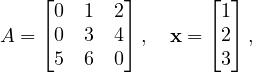
One example A,x could be:
for which, if the exercise is implemented OK, the output would be something like:
Step 1: Constructing a 3x3 sparse matrix A.
Step 2: Creating vector x = [1, 2, 3]^T.
Step 3: Computing y = A⋅x under plus-times semiring.
Step 4: Computing z = x ⊙ y (element-wise multiply).
Step 5: Computing dot_val = x⊤⋅x under plus-times semiring.
x = [ 1, 2, 3 ]
y = A⋅x = [ 8, 18, 17 ]
z = x ⊙ y = [ 8, 36, 51 ]
dot(x,x) = 14
Question. If setting all n elements of a size-n vector via grb::setElement, what is its big-Omega (lower-bound
asymptotic) complexity? Is the resulting complexity reasonable for a shared-memory parallel program?
Bonus question. If instead those n elements are in some STL-type container for which we retrieve random
access iterators, and ingest those elements using grb::buildVectorUnique and those random access
iterators – what would a good shared-memory parallel ALP/GraphBLAS implementation achieve in terms of
complexity ?
From these questions it follows that grb::setElement should only ever be used to set Θ(1) elements in some
container and never asymptotically more than that. If a larger data set needs to be ingested into ALP
containers, then in order to guarantee scalability, always rely on (parallel) iterators and the grb::build*
primitives!
3.5 Semirings and Algebraic Operations
A key feature of GraphBLAS and ALP is that operations are defined over generic algebraic structures rather than over
the conventional arithmetic operations only. An example of an algebraic structure is a semiring. Loosely
speaking, a semiring formalises what we understand as standard linear algebra. Intuitively, a semiring
consists of a pair of operations, an “addition” and a “multiplication”, along with their identity elements. The
additive and multiplicative operations may differ from standard arithmetic (+ and ×). The multiplicative
operation together with its identity – which we call 1 – forms a monoid. The additive operation together with
its identity – 0 – forms a commutative monoid, meaning that the order of addition shall not change the
result (a + b = b + a). Formally speaking there are more requirements to monoids and semirings that ALP
is aware of and exploits – however, for the purposes of this tutorial, the preceding intuitive description
suffices.
GraphBLAS allows using different semirings to, for example, perform computations like shortest paths or logical
operations by substituting the plus or times operations with min, max, logical OR/AND, and so on. This is usually done
structurally, by replacing the plus-times semirings with another, such as e.g. a min-plus semiring to compute shortest
paths. This is why, as you saw in the previous subsection, GraphBLAS primitives explicitly take algebraic structures as a
mandatory argument. ALP additionally allows expressing algebraic structures as C++ types, and introduces an algebraic
type trait system:
-
commutative monoids: an associative and commutative operation with an identity element. Examples:
-
(+, 0) — the usual addition over numbers:
grb::Monoid< grb::operators::add< T >, grb::identities::zero >
or, more simply,
grb::monoids::plus< T >
-
(min, ∞) — useful for computing minima:
grb::Monoid< grb::operators::min< T >, grb::identities::infinity > // or simply
grb::monoids::min< T >
-
(∧, true) — logical semiring for Boolean algebra:
grb::Monoid< grb::operators::logical_and >, grb::identities::logical_true > // or
grb::monoids:land< T >
For all the above examples, the following type traits are true:
grb::is_monoid< grb::monoid::plus< T > >::value
grb::is_commutative< grb::monoid::min< T > >::value
// and so on
-
general binary operators: binary operators without any additional structure. Examples:
grb::operators::mul< double >    // f(x, y) = x * y
grb::operators::subtract< int >  // f(i, j) = i - j
grb::operators::zip< char, int > // f(c, i) = {c, i}, an std::pair< char, int >
These too define algebraic type traits:
grb::is_operator< OP >::value // true for all above operators
grb::is_monoid< OP >::value   // false for all above operators
grb::is_associative< grb::operators::mul< T > >::value    // true
grb::is_commutative< grb::operators::subtract< T >::value // false
// ...
-
semirings: simplified, a commutative “additive” monoid combined with a “multiplicative” monoid. Examples:
-
the plus-times semiring: standard linear algebra
grb::Semiring<
    grb::operators::add< T >, grb::operators::mul< T >,
    grb::identities::zero, grb::identities::one
> // or
grb::semirings::plusTimes< T >
-
the Boolean semiring: perhaps the second most common semiring
grb::Semiring<
    grb::operators::logical_or< bool >, grb::operators::logical_and< bool >,
    grb::identities::logical_false, grb::identities::logical_true
> // or
grb::semirings::boolean
-
the min-plus semiring: useful for, e.g., shortest paths
grb::Semiring<
    grb::operators::min< T >, grb::operators::add< T >,
    grb::identities::infinity, grb::identities::zero
> // or
grb::semirings:::minPlus< T >
For all of the above semirings, we have the following:
grb::is_semiring< S >::value // true
grb::is_monoid< S >::value   // false
grb::is_operator< S >::value // false
We may furthermore extract the additive and multiplicative monoids and operators from semirings:
grb::semirings::boolean mySemiring;
auto myAddM  = mySemiring.getAdditiveMonoid();
auto myMulM  = mySemiring.getMultiplicativeMonoid();
auto myAddOp = mySemiring.getAdditiveOperator();
auto myMulOp = myMulM.getOperator();
Finally, we may also extract and instantiate identities from semirings:
grb::semirings::plusTimes< int > mySemiring;
constexpr int myZero = mySemiring.template getZero< int >();
double castFromZero = mySemiring.template getZero< double >();
constexpr int myOne = mySemiring.getMultiplicativeMonoid().template getIdentity();
The design of ALP allows the definition of custom operators and identities, and therefore allows a virtually unlimited
variety of algebraic structures. The most useful operators, monoids, and semirings are predefined in the
namespaces grb::operators, grb::monoids, and grb::semirings, respectively. Let us now employ
these algebraic structures to show-case how these amplify the expressiveness of standard linear algebraic
primitives.
Exercise 9 (warm-up): given a grb::Vector< double > x, write an ALP/GraphBLAS function that computes the
squared 2-norm of x (i.e., compute ∑
ixi2) using grb::dot. Hint: consider starting from the code of exercise 8.
Question: which semiring applies here?
Exercise 10: ALP and GraphBLAS allow for the use of improper semirings – semirings that are mathematically not true
semirings but are still useful in practice. In ALP, improper semirings are made up of 1) an commutative “additive”
monoid and 2) any binary “multiplicative” operator. All primitives that take a semiring may also take a pair of such an
additive monoid and multiplicative operator– for example, grb::dot( alpha, x, y, plusTimes ) is semantically
equivalent to
grb::dot( alpha, x, y, plusTimes.getAdditiveMonoid(), plusTimes.getMultiplicativeOperator() );
Take note of grb::operators::abs_diff< double >. What does this binary operator compute? Use this
operator and the notion of improper semirings to compute the 1-norm difference between two vectors x and y using a
single call to grb::dot. Hint: start off from the code from the previous exercise.
Exercise 11: consider a square matrix grb::Matrix< double > G the matrix representation of an
edge-weighted graph G. Consider grb::Vector< double > s (source) a vector of matching dimension
to G with a single value zero (0) at an index of your choosing. Question: normally, under a plusTimes
semiring, Gs would return a zero vector. However, what interpretation would Gs have under the minPlus
semiring? Use this interpretation to compute the shortest path to any other vertex reachable from your
chosen source. Then, extend the approach to compute the shortest path two hops away from your chosen
source.
Bonus question: what interpretation could Gks have under the maxTimes semiring?
4 Solution to Exercise 8
Below a sample solution code for this example, with
commentary:
/*
 * example.cpp - Corrected minimal ALP (GraphBLAS) example.
 *
 * To compile (using the reference OpenMP backend):
 *    grbcxx -b reference_omp example.cpp -o example
 *
 * To run:
 *    grbrun ./example
 */

#include <cstdio>
#include <iostream>
#include <vector>
#include <utility>   // for std::pair
#include <array>

#include <graphblas.hpp>

using namespace grb;

// Indices and values for our sparse 3x3 matrix A:
//
//      A = [ 1   0   2 ]
//          [ 0   3   4 ]
//          [ 5   6   0 ]
//
// We store the nonzero entries via buildMatrixUnique.
static const size_t Iidx[6]    = { 0, 0, 1, 1, 2, 2 };  // row indices
static const size_t Jidx[6]    = { 0, 2, 1, 2, 0, 1 };  // column indices
static const double Avalues[6] = { 1.0, 2.0, 3.0, 4.0, 5.0, 6.0 };

int main( int argc, char **argv ) {
    (void)argc;
    (void)argv;
    std::printf("example (ALP/GraphBLAS) API usage\n\n");

    //------------------------------
    // 1) Create a 3x3 sparse matrix A
    //------------------------------
    std::printf("Step 1: Constructing a 3x3 sparse matrix A.\n");
    Matrix<double> A(3, 3);
    // Reserve space for 6 nonzeros
    resize(A, 6);
    // Populate A from (Iidx,Jidx,Avalues)
    buildMatrixUnique(
        A,
        &(Iidx[0]),
        &(Jidx[0]),
        Avalues,
        /* nvals = */ 6,
        SEQUENTIAL
    );

    //------------------------------
    // 2) Create a 3-element vector x and initialize x = [1, 2, 3]^T
    //------------------------------
    std::printf("Step 2: Creating vector x = [1, 2, 3]^T.\n");
    Vector<double> x(3);
    set<descriptors::no_operation>(x, 0.0);           // zero-out
    setElement<descriptors::no_operation>(x, 1.0, 0); // x(0) = 1.0
    setElement<descriptors::no_operation>(x, 2.0, 1); // x(1) = 2.0
    setElement<descriptors::no_operation>(x, 3.0, 2); // x(2) = 3.0
    // note: setElement() supports vectors only
    //       set() support for matrix is work in progress

    //------------------------------
    // 3) Create two result vectors y and z (dimension 3)
    //------------------------------
    Vector<double> y(3), z(3);
    set<descriptors::no_operation>(y, 0.0);
    set<descriptors::no_operation>(z, 0.0);

    //------------------------------
    // 4) Use the built-in "‘plusTimes’" semiring alias
    //      (add = plus, multiply = times, id-add = 0.0, id-mul = 1.0)
    //------------------------------
    auto plusTimes = grb::semirings::plusTimes<double>();

    //------------------------------
    // 5) Compute y = A⋅x  (matrix-vector multiply under plus-times)
    //------------------------------
    std::printf("Step 3: Computing y = A⋅x under plus-times semiring.\n");
    {
        RC rc = mxv<descriptors::no_operation>(y, A, x, plusTimes);
        if(rc != SUCCESS) {
            std::cerr << "Error: mxv(y,A,x) failed with code " << toString(rc) << "\n";
            return (int)rc;
        }
    }

    //------------------------------
    // 6) Compute z = x ⊙ y  (element-wise multiply) via eWiseMul with semiring
    //------------------------------
    std::printf("Step 4: Computing z = x ⊙ y (element-wise multiply).\n");
    {
        RC rc = eWiseMul<descriptors::no_operation>(
            z, x, y, plusTimes
        );
        if(rc != SUCCESS) {
            std::cerr << "Error: eWiseMul(z,x,y,plusTimes) failed with code " << toString(rc) << "\n";
            return (int)rc;
        }
    }

    //------------------------------
    // 7) Compute dot_val = x⊤⋅x  (dot-product under plus-times semiring)
    //------------------------------
    std::printf("Step 5: Computing dot_val = x⊤⋅x under plus-times semiring.\n");
    double dot_val = 0.0;
    {
        RC rc = dot<descriptors::no_operation>(dot_val, x, x, plusTimes);
        if(rc != SUCCESS) {
            std::cerr << "Error: dot(x,x) failed with code " << toString(rc) << "\n";
            return (int)rc;
        }
    }

    //------------------------------
    // 8) Print x, y, z, and dot_val
    //    We reconstruct each full 3 - vector by filling an std::array<3,double>
    //------------------------------
    auto printVector = [&](const Vector<double> &v, const std::string &name) {
        // Initialize all entries to zero
        std::array<double,3> arr = { 0.0, 0.0, 0.0 };
        // Overwrite stored (nonzero) entries
        for(const auto &pair : v) {
            // pair.first = index, pair.second = value
            arr[pair.first] = pair.second;
        }
        // Print
        std::printf("%s = [ ", name.c_str());
        for(size_t i = 0; i < 3; ++i) {
            std::printf("%g", arr[i]);
            if(i + 1 < 3) std::printf(", ");
        }
        std::printf(" ]\n");
    };

    std::printf("\n-- Results --\n");
    printVector(x, "x");
    printVector(y, "y = A⋅x");
    printVector(z, "z = x ⊙ y");
    std::printf("dot(x,x) = %g\n\n", dot_val);

    return EXIT_SUCCESS;
}
Listing 1:
Example
program
using
ALP/GraphBLAS
primitives
in
C++
The expected output is (bash)
example (ALP/GraphBLAS) corrected API usage

Step 1: Constructing a 3x3 sparse matrix A.
Step 2: Creating vector x = [1, 2, 3]^T.
Step 3: Computing y = A⋅x under plus-times semiring.
Step 4: Computing z = x ⊙ y (element-wise multiply).
Step 5: Computing dot_val = x⊤⋅x under plus-times semiring.

-- Results --
x = [ 1, 2, 3 ]
y = A⋅x = [ 7, 18, 17 ]
z = x ⊙ y = [ 7, 36, 51 ]
dot(x,x) = 14
$
4.1 Makefile and CMake Instructions
Finally, we provide guidance on compiling and running the above example in your own development environment. If you
followed the installation steps and used grbcxx, compilation is straightforward. Here we outline two approaches: using
the ALP wrapper scripts, and integrating ALP manually via a build system.
Using the ALP compiler wrapper
The simplest way to compile your ALP-based program is to use the provided wrapper. After sourcing the ALP
environment (setenv script), the commands grbcxx and grbrun are available in your PATH. You can compile the
example above by saving it (e.g. as example.cpp) and running:
$ grbcxx example.cpp -o example
This will automatically invoke g++ with the correct include directories and link against the ALP library
and its required libraries (NUMA, pthread, etc.). By default, it uses the sequential backend. To enable
parallel execution with OpenMP, add the flag -b reference_omp (for shared-memory parallelism). For
instance:
$ grbcxx -b reference_omp example.cpp -o example
After compilation, run the program with:
$ grbrun ./example
(You can also run ./example directly for a non-distributed run; grbrun is mainly needed for orchestrating
distributed runs or setting up the execution environment.)
Using a custom build (Make/CMake)
If you prefer to compile without the wrapper (for integration into an existing project or custom build system), you need
to instruct your compiler to include ALP’s headers and link against the ALP library and dependencies. The ALP
installation (at the chosen -prefix) provides an include directory and a library directory.
For example, if ALP is installed in ../install as above, you could compile the program manually with:
$ g++ -std=c++17 example.cpp
-I../install/include -D_GRB_WITH_REFERENCE -D_GRB_WITH_OMP -L../install/lib/sequential
-lgraphblas -lnuma -lpthread -lm -fopenmp -o example
Here we specify the include path for ALP headers and link with the ALP GraphBLAS library (assumed to be named
libgraphblas) as well as libnuma, libpthread, libm (math), and OpenMP (the -fopenmp flag). These additional
libraries are required by ALP (as noted in the install documentation). Using this command (or a corresponding Makefile
rule) will produce the executable example.
If you are using CMake for your own project, you can integrate ALP as follows. There may not be an official
CMake package for ALP, but you can use find_library or hard-code the path. For instance, in your
CMakeLists.txt:
    cmake_minimum_required(VERSION 3.13)
    project(ALPExample CXX)
    find_package(OpenMP REQUIRED) # find OpenMP for -fopenmp
    set(ALP_PREFIX "../install") # Adjust ../install to your ALP installation prefix
    include_directories("${ALP_PREFIX}/include")
    link_directories("${ALP_PREFIX}/lib" "${ALP_PREFIX}/lib/sequential")
    add_executable(example example.cpp)
    target_compile_options(example PRIVATE -O3 -march=native -std=c++17 -D_GRB_WITH_REFERENCE -D_GRB_WITH_OMP)
    target_link_libraries(example graphblas numa pthread m OpenMP::OpenMP_CXX)
Listing 2:
Example
CMakeLists.txt
for
an
ALP
project
This will ensure the compiler knows where to find graphblas.hpp and links the required libraries. After configuring
with CMake and building (via make), you can run the program as usual.
Note: If ALP provides a CMake package file, you could use find_package for ALP, but at the time of writing,
linking manually as above is the general approach. Always make sure the library names and paths correspond to your
installation. The ALP documentation mentions that programs should link with -lnuma, -lpthread, -lm, and OpenMP
flags in addition to the ALP library.
This tutorial has introduced the fundamentals of using ALP/GraphBLAS in C++ on Linux, from installation to
running a basic example. With ALP set up, you can explore more complex graph algorithms and linear algebra
operations, confident that the library will handle parallelization and optimization under the hood. Happy
coding!
5 ALP Transition Paths
Algebraic Programming (ALP) is a C++ framework for high-performance linear algebra that can auto-parallelize
and auto-optimize your code. A key feature of ALP is its transition path APIs, which let you use ALP through standard
interfaces without changing your existing code. In practice, ALP generates drop-in replacements for established linear
algebra APIs. You simply re-link your program against ALP’s libraries to get optimized performance (no code
modifications needed). ALP v0.8 provides transition-path libraries for several standards, including the NIST Sparse BLAS
and a CRS-based iterative solver interface (ALP/Solver). This means you can take an existing C/C++ program that uses
a supported API and benefit from ALP’s optimizations (such as vectorization and parallelism) just by linking with ALP’s
libraries [1].
One of these transition paths, and the focus of this tutorial, is ALP’s sparse Conjugate Gradient (CG) solver.
This CG solver accepts matrices in Compressed Row Storage (CRS) format (also known as CSR) and solves Ax = b using
an iterative method. Under the hood it leverages ALP’s non-blocking execution model, which overlaps computations and
memory operations for efficiency. From the user’s perspective, however, the solver is accessed via a simple
C-style API that feels synchronous. In this workshop, we’ll learn how to use this CG solver interface step by
step: from setting up ALP, to coding a solution for a small linear system, to building and running the
program.
5.1 Setup: Installing ALP and Preparing to Use the Solver
This section explains how to install ALP on a Linux system and compile a simple example. ALP (Algebraic
Programming) provides a C++17 library implementing the GraphBLAS interface for linear-algebra-based
computations.
Installation on Linux
- Install prerequisites: Ensure you have a C++11 compatible compiler (e.g. g++ 4.8.2 or later) with OpenMP
support, CMake (>= 3.13) and GNU Make, plus development headers for libNUMA and POSIX threads.
For example, on Debian/Ubuntu:
sudo apt-get install build-essential libnuma-dev libpthread-stubs0-dev cmake
Direct linking option: If you prefer to compile with your usual compiler, you need to include ALP’s
headers and link against the ALP libraries manually. For the CG solver transition path, that typically means
linking against the sparse solver library (e.g. libspsolver_shmem_parallel for the parallel version) and
any core ALP libraries it depends on. For example, if ALP is installed in /opt/alp, you might compile
with:
gcc -I/opt/alp/include -L/opt/alp/lib \
-lspsolver_shmem_parallel -lalp_cspblas_shmem_parallel \
my_program.c -o my_program
(ALP’s documentation provides details on which libraries to link for each backend [3].) Using grbcxx is recommended
for simplicity, but it’s good to know what happens under the hood. Now that our environment is set up, let’s look at the
CG solver API.
5.2 Overview of ALP’s Non-Blocking Sparse CG API
The ALP/Solver transition path provides a C-style interface for initializing and running a Conjugate Gradient solver. All
functions are exposed via a header (e.g. solver.h in ALP’s include directory) and use simple types like pointers and
handles. The main functions in this API are:
- sparse_cg_init(&handle, n, vals, cols, offs): Initializes a CG solver instance. It allocates/assigns a
solver context to the user-provided sparse_cg_handle_t (an opaque handle type defined by ALP). The
matrix A is provided in CRS format by three arrays: vals (the nonzero values), cols (the column indices for
each value), and offs (offsets in the vals array where each row begins). The dimension n (number of rows,
which should equal number of columns for A) is also given. After this call, the handle represents an internal
solver state with matrix A stored. Return: Typically returns 0 on success (and a non-zero error code on
failure) [4].
- sparse_cg_set_preconditioner(handle, func, data): (Optional) Sets a preconditioner for the iterative
solve. The user provides a function func that applies the preconditioner M−1 to a vector (i.e. solves Mz = r
for a given residual r), along with a user data pointer. ALP will call this func(z, r, data) in each CG iteration
to precondition the residual. If you don’t call this, the solver will default to no preconditioning (i.e. M = I).
You can use this to plug in simple preconditioners (like Jacobi, with data holding the diagonal of A) or
even advanced ones, without modifying the solver code. Return: 0 on success, or error code if the handle is
invalid, etc.
- sparse_cg_solve(handle, x, b): Runs the CG iteration to solve Ax = b. Here b is the right-hand side
vector (input), and x is the solution vector (output). You should allocate both of these arrays of length n
beforehand. The solver will iterate until it converges to a solution within some default tolerance or until
it reaches an iteration limit. On input, you may put an initial guess in x. If not, it’s safe to initialize x to
zero (the solver will start from x0 = 0 by default in that case). Upon return, x will contain the approximate
solution. Return: 0 if the solution converged (or still 0 if it ran the maximum iterations – specific error codes
might indicate divergence or other issues in future versions).
- sparse_cg_destroy(handle): Destroys the solver instance and releases any resources associated with the
given handle. After this, the handle becomes invalid. Always call this when you are done solving to avoid
memory leaks. Return: 0 on success (and the handle pointer may be set to NULL or invalid after). This
API is non-blocking in the sense that internally ALP may overlap operations (like sparse matrix-vector
multiplications and vector updates) and use asynchronous execution for performance. However, the above
functions themselves appear synchronous. For example, sparse_cg_solve will only return after the solve
is complete (there’s no separate “wait” call exposed in this C interface). The benefit of ALP’s approach is
that you, the developer, don’t need to manage threads or message passing at all ALP’s GraphBLAS engine
handles parallelism behind the scenes. You just call these routines as you would any standard library. Now,
let’s put these functions into practice with a concrete example.
This API is non-blocking in the sense that internally ALP may overlap operations (like sparse matrix-vector
multiplications and vector updates) and use asynchronous execution for performance. However, the above functions
themselves appear synchronous. For example, sparse_cg_solve will only return after the solve is complete (there’s no
separate “wait” call exposed in this C interface). The benefit of ALP’s approach is that you, the developer, don’t need to
manage threads or message passing at all. ALP’s GraphBLAS engine handles parallelism behind the scenes. You just call
these routines as you would any standard library. Now, let’s put these functions into practice with a concrete
example.
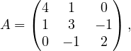
5.3 Example: Solving a Linear System with ALP’s CG Solver
Suppose we want to solve a small system Ax = b to familiarize ourselves with the CG interface. We will use the following
3 × 3 symmetric positive-definite matrix A:
and we choose a right-hand side vector b such that the true solution is easy to verify. If we take the solution to be
x = (1, 2, 3), then b = Ax can be calculated as:
since 4 ⋅ 1 + 1 ⋅ 2 + 0 ⋅ 3 = 6, 1 ⋅ 1 + 3 ⋅ 2 + (−1) ⋅ 3 = 4, and 0 ⋅ 1 + (−1) ⋅ 2 + 2 ⋅ 3 = 4. Our goal is to see if the CG solver
recovers x = (1,2,3) from A and b.
We will hard-code A in CRS format (also called CSR: Compressed Sparse Row) for the solver. In CRS, the matrix is
stored by rows, using parallel arrays for values and column indices, plus an offset index for where each row starts. For
matrix A above:
- Nonzero values in row 0 are [4, 1] (at columns 0 and 1), in row 1 are [1, 3, -1] (at cols 0,1,2), and in row 2
are [-1, 2] (at cols 1,2). So the vals array will be {4, 1, 1, 3, -1, -1, 2} (concatenated by row).
- Corresponding column indices cols would be {0, 1, 0, 1, 2, 1, 2} aligned with each value.
- The offsets offs marking the start of each row’s data in the vals array would be: row0 starts at index 0, row1
at index 2, row2 at index 5, and an extra final entry = 7 (total number of nonzeros). So offs = {0, 2, 5, 7}.
Below is a complete program using ALP’s CG solver to solve for x. We include the necessary ALP
header for the solver API, set up the matrix and vectors, call the API functions in order, and then print the
result.
#include <stdio.h>
#include <stdlib.h>

// Include ALPs solver API header
#include <transition/solver.h> // (path may vary based on installation)

int main(){
    // Define the 3x3 test matrix in CRS format
    const size_t n = 3;

    double A_vals[] = {
        4.0, 1.0, // row 0 values
        1.0, 3.0, -1.0, // row 1 values
        -1.0, 2.0 // row 2 values
    };

    int A_cols[] = {
        0, 1, // row 0 column indices
        0, 1, 2, // row 1 column indices
        1, 2 // row 2 column indices
    };

    int A_offs[] = { 0, 2, 5, 7 }; // row start offsets: 0,2,5 and total nnz=7

    // Right-hand side b and solution vector x
    double b[] = { 6.0, 4.0, 4.0 }; // b = A * [1,2,3]^T
    double x[] = { 0.0, 0.0, 0.0 }; // initial guess x=0 (will hold the solution)

    // Solver handle
    sparse_cg_handle_t handle;

    int err = sparse_cg_init_dii(&handle, n, A_vals, A_cols, A_offs);
    if (err != 0) {
        fprintf(stderr, "CG init failed with error %d\n", err);
        return EXIT_FAILURE;
    }

    // (Optional) set a preconditioner here if needed, e.g. Jacobi or others.
    // We skip this, so no preconditioner (effectively M = Identity).
    err = sparse_cg_solve_dii(handle, x, b);
    if (err != 0) {
        fprintf(stderr, "CG solve failed with error %d\n", err);
        // Destroy handle before exiting
        sparse_cg_destroy_dii(handle);
        return EXIT_FAILURE;
    }

    // Print the solution vector x
    printf("Solution x = [%.2f, %.2f, %.2f]\n", x[0], x[1], x[2]);

    // Clean up
    sparse_cg_destroy_dii(handle);

    return 0;
}
Listing 3:
Example
program
using
ALP’s
CG
solver
API
Let’s break down what happens here:
- We included <graphblas/solver.h> (the exact include path might be alp/solver.h or similar depending on
ALP’s install, but typically it resides in the GraphBLAS include directory of ALP). This header defines the
sparse_cg_* functions and the sparse_cg_handle_t type.
- We set up the matrix data in CRS format. For clarity, the values and indices are grouped by row in the
code. The offsets array {0,2,5,7} indicates: row0 uses vals[0..1], row1 uses vals[2..4] , row2 uses vals[5..6].
The matrix dimension n is 3.
- We prepare the vectors b and x. b is initialized to {6,4,4} as computed above. We initialize x to all zeros (as
a starting guess). In a real scenario, you could start from a different guess, but zero is a common default.
- We create a sparse_cg_handle_t and call sparse_cg_init. This hands the matrix to ALP’s solver. Under
the hood, ALP will likely copy or reference this data and possibly analyze A for the CG algorithm. We
check the return code err, if non-zero, we print an error and exit. (For example, an error might occur if n
or the offsets are inconsistent. In our case, it should succeed with err == 0.)
- We do not call sparse_cg_set_preconditioner in this example, which means the CG will run
unpreconditioned. If we wanted to, we could implement a simple preconditioner. For instance, a Jacobi
preconditioner would use the diagonal of A: we’d create an array with diag(A) = [4,3,2] and a function
to divide the residual by this diagonal. We would then call sparse_cg_set_preconditioner(handle,
my_prec_func, diag_data). For brevity, we skip this. ALP will just use the identity preconditioner by
default (no acceleration).
- Next, we call sparse_cg_solve(handle, x, b). ALP will iterate internally to solve Ax = b. When this
function returns, x should contain the solution. We again check err. A non-zero code could indicate the
solver failed to converge (though typically it would still return 0 and one would check convergence via a
status or residual, ALP’s API may evolve to provide more info). In our small case, it should converge in at
most 3 iterations since A is 3 × 3.
- We print the resulting x. We expect to see something close to [1.00, 2.00, 3.00]. Because our matrix and b were
consistent with an exact solution of (1,2,3), the CG method should find that exactly (within floating-point
rounding). You can compare this output with the known true solution to verify the solver worked correctly.
- Finally, we call sparse_cg_destroy(handle) to free ALP’s resources for the solver. This is important
especially for larger problems to avoid memory leaks. After this, we return from main.
Building and Running the Example
To compile the above code with ALP, we will use the direct linking option as discussed.
g++ example.cpp -o cg_demo \
-I$ALP_INSTALL_DIR/include \
-L$ALP_INSTALL_DIR/lib/ -L$ALP_INSTALL_DIR/lib/sequential/ \
-lspsolver_shmem_parallel -lgraphblas -fopenmp -lnuma
After a successful compile, you can run the program:
    export LD_LIBRARY_PATH=$LD_LIBRARY_PATH:$ALP_INSTALL_DIR/lib:$ALP_INSTALL_DIR/lib/sequential/
    ./cg_demo
It should output something like:
Solution x = [1.00, 2.00, 3.00]
Congratulations! You’ve now written and executed a Conjugate Gradient solver using ALP’s transition path API! By
using this C-style interface, we got the benefits of ALP’s high-performance GraphBLAS engine without
having to dive into template programming or parallelization details. From here, you can explore other
parts of ALP’s API: for instance, ALP/GraphBLAS provides a full GraphBLAS-compatible API for linear
algebra operations on vectors and matrices, and ALP also offers a Pregel-like graph processing interface.
All of these can be integrated with existing code in a similar fashion (just link against ALP’s libraries)
[2][3].
In summary, ALP’s transition paths enable a smooth adoption of advanced HPC algorithms – you write standard
code, and ALP handles the rest. We focused on the CG solver, but the same idea applies to other supported interfaces.
Feel free to experiment with different matrices, add a custom preconditioner function to see its effect, or try other solvers
if ALP introduces them in future releases. Happy coding!
References
6 Advanced ALP
This Section treats some more advanced ALP topics by which programmers can exercise tighter control over performance
or semantics.
We have previously seen that the semantics of primitives may be subtly changed by the use of descriptors: e.g., adding
grb::descriptors::transpose_matrix to grb::mxv has the primitive interpret the given matrix A as its
transpose (AT) instead. Other descriptors, however, may also modify the performance semantics of a primitive. One
example is the grb::descriptors::dense descriptor, which has two main effects when supplied to a
primitive:
- all vector arguments to the primitive must be dense on primitive entry; and
- any code paths that check sparsity or deal with sparsity are disabled.
The latter effect directly affects performance, which is particularly evident for the grb::nonblocking backend.
Another type of performance effect also caused by the latter is that produced binary code is smaller in size as
well.
Exercise 12: inspect the implementation of the PCG method in ALP. Run experiments using the nonblocking
backend, comparing the performance of repeated linear solves with and without the dense descriptor. Also inspect the size
of the binary. Hint: try make -j\$(nprocs) build_tests_category_performance and see if an executable is
produced in tests/performance that helps you complete this exercise faster.
6.2 Explicit SPMD
When compiling any ALP program with a distributed-memory backend such as bsp1d or hybrid, ALP automatically
parallelises across multiple user processes. Most of the time this suffices, however, in some rare cases, the ALP
programmer requires exercising explicit control over distributed-memory parallelism. Facilities for these exist across
three components, in order of increasing control: grb::spmd, grb::collectives, and explicit backend
dispatching.
Basic SPMD
When selecting a distributed-memory backend, ALP automatically generates SPMD code without the user having to
intervene. The grb::spmd class exposes these normally-hidden SPMD constructs to the programmer: 1)
grb::spmd<>::nprocs() returns the number of user processes in the current ALP program, while 2)
grb::spmd<>::pid() returns the unique ID of the current user process.
Exercise 13: try to compile and run the earlier hello-world example using the bsp1d backend. How many hello world
messages are printed? Hint: use -np 2 to grbrun to spawn two user processes when executing the program. Now
modify the program so that no matter how many user processes are spawned, only one message is printed to the screen
(stdout).
Collectives
The most common way to orchestrate data movement between user processes are the so-called collective communications.
Examples include:
- broadcast, a communication pattern where one of the user processes is designated the root of the
communication, and has one payload message that should materialise on all other user processes.
- allreduce, a communication pattern where all user processes have a value that should be reduced into a single
aggregate value, which furthermore must be available at each user process.
ALP also exposes collectives, and in the case of (all)reduce does so in an algebraic manner– that is,
the signature of an allreduce expects an explicit monoid that indicates how aggregation is supposed to
occur:
size_t to_be_reduced = grb::spmd<>::pid();;
grb::monoid::max< int > max;
grb::RC rc = grb::collectives<>::allreduce( to_be_reduced, max );
if( rc == grb::SUCCESS ) { assert( to_be_reduced + 1 == grb::spmd<>::nprocs ); }
if( grb::spmd<>::pid() == 0 ) { std::cout << "There are " << to_be_reduced << " processes\n"; }
Exercise 14: change the initial assignment of to_be_reduced to 1 (at each process). Modify the above example to still
compute the number of processes via an allreduce collective. Hint: if aggregation by the max-monoid is not suitable after
changing the initialised value, which aggregator would be?
Explicit dispatching
ALP containers are templated in the backend they are compiled for– this is specified as the second template argument,
which is default-initialised to the backend given to the grbcxx wrapper. This means the backend is part of the type of
ALP containers, which, in turn, enables the compiler to generate, for each ALP primitive, the code that corresponds to
the requested backend. It is, however, possible to manually override this backend template argument, which is useful in
conjunction with SPMD in that the combination allows the programmer to define operations that should
execute within a user process only, as opposed to defining operations that should be performed across user
processes.
For example, within a program compiled with the bsp1d or hybrid backends, a user may define a process-local
vector as follows: grb::Vector< double, grb::nonblocking > local_x( local_n ), where local_n is
some local size indicator that normally is proportional to n∕P, with n a global size and P the total number of
user processes. Using grb::spmd, the programmer may specify that each user process performs different
computations on their local vectors. This results in process-local computations that are totally independent of
other processes, which later on may be aggregated into some meaningful global state through, for example,
collectives.
Exercise 15: use the mechanism here described to write a program that, when executed using P processes,
solves P different linear systems Ax = bk where A is the same at every process while the bk, 0 ≤ k < P
are initialised to (k,k,…,k)T each. Make it so that the program returns the maximum residual (squared
2-norm of b − Ax) across the P processes. Hint: reuse one of the pre-implemented linear solvers, such as
CG.
Acknowledgements
This document was compiled from LaTeX source code using GitHub Actions and deployed to GitHub
Pages.
This document was generated on December 2, 2025.